Introduction

When I was writing my master thesis^[1] I wanted the figures to look professional, meaning I wanted at least the same font in the figure as used all over my document. However, TikZ^[2] was not an option, because I wanted to focus on the actual programming (and signal processing) tasks and not too much on my love for beautiful documents in the little time I was given. I searched the world wide web and I had a Morpheus moment when I came across the inkscape^[3] --export-latex option.

Sounds pretty good, right? The suggested workflow with inkscape is a follows.

Create a SVG w/ Python

Let's get our hands dirty right away. As a first step an image needs to be created. Theoretically, it does not matter how the SVG is produced. I tried Python and draw.io.

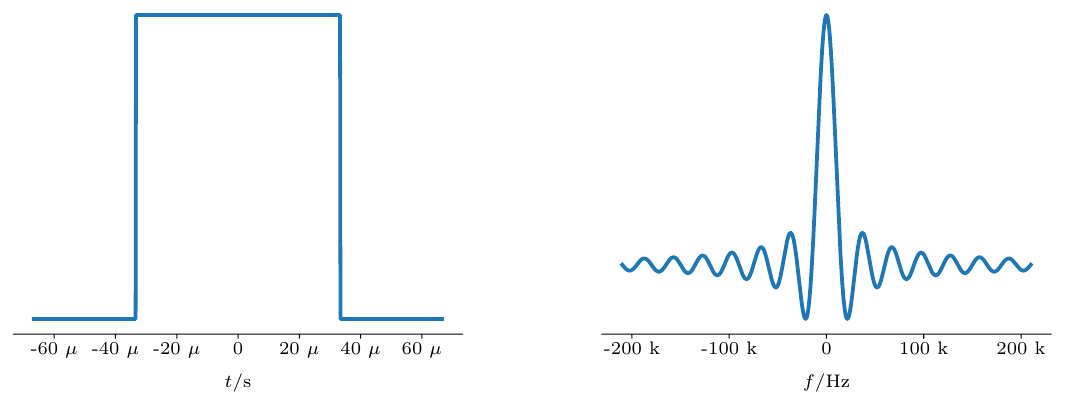
The image decorating this post is a screenshot of a LaTeX compiled PDF. To give an example, I am going to show how to make those two plots leveraging Python in conjuction with matplotlib^[4]. Here comes an excerpt of the code, which created those two waveforms.

from matplotlib import pyplot as plt
import numpy as np
from matplotlib.ticker import EngFormatter

# Settings
plt.rcParams['font.size'] = 12
plt.rcParams['svg.fonttype'] = 'none'

# Master thesis colors
color0 = '#00285e'

# Sexy formatter engineering style
formatter0 = EngFormatter(unit='')
formatter1 = EngFormatter(unit='s')

w = float(1)/15e3
carriers = 12
x = np.linspace(-15e3*(carriers+2),15e3*(carriers+2),1000)

# Single carrier
b = np.sinc(x*w)
plt.plot(x,b,label="\$\\frac{sin(f)}{f}\$", linewidth=3, color=color0)

# Plot formatting
axes = plt.gca()
axes.xaxis.set_major_formatter(formatter0)
axes.set_xlabel("\$f/\SI{}{\Hz}\$")
for side in ['right','top','left']:
  axes.spines[side].set_visible(False)
axes.xaxis.labelpad = 15
axes.yaxis.labelpad = 15
plt.title("Single \gls{NB-IoT} Sub-Carrier")
plt.yticks([])
plt.savefig("ofdm_nbiot_sinc.svg", format="svg", transparent=True)
plt.clf()

# Pulse shape
t = np.linspace(-(1/15e3), 1/15e3, 1000)
boxcar = [0]*(len(t)/4) + [1]*(len(t)/2) + [0]*(len(t)/4)
plt.plot(t,boxcar,label="\$s(t)\$", linewidth=3, color=color0)

# Plot formatting
axes = plt.gca()
axes.set_xlabel("\$t/\SI{}{\second}\$")
axes.xaxis.set_major_formatter(formatter0)
for side in ['right','top','left']:
  axes.spines[side].set_visible(False)
axes.xaxis.labelpad = 15
axes.yaxis.labelpad = 15
plt.title("\gls{NB-IoT} Pulse-Shape")
plt.yticks([])
plt.savefig("ofdm_nbiot_boxcar.svg", format="svg", transparent=True)
plt.clf()

Now there are two SVGs in that directory, which can be further processed.

Converting the SVG to LaTeX

The second step is pretty straight forward. Once you have a .svg file. You can feed it into inkscape and their great plugin will take care of (almost) all the rest.

inkscape -D --export-latex --export-filename=./figs/ofdm_nbiot_boxcar.pdf ./figs/ofdm_nbiot_boxcar.svg

As one can see, in that case all figures are stored in a directory called figs. This might concern you, since you found out, that the produced .pdf_tex file references to ofdm_nbiot_boxcar.pdf directly. I fixed this issue by calling rpl, a neat program to replace strings in files.

rpl -q ofdm_nbiot_boxcar.pdf ./figs/ofdm_nbiot_boxcar.pdf ./figs/ofdm_nbiot_boxcar.pdf_tex

Fixed it! Basically, you could also open the .pdf_tex output file in a standard editor and just find & replace every occurance (if you have nothing else to do).

Interfacing w/ LaTeX

All you need to do next is to include the following lines into your LaTeX document.

\begin{figure}[htbp]
  \begin{subfigure}{0.49\columnwidth}
    \centering
    \scriptsize
    \def\svgwidth{\columnwidth}
    \input{./figs/ofdm_nbiot_boxcar.pdf_tex}
    \caption{}
    \label{fig:ofdm_nbiot_boxcar}
  \end{subfigure}
  \begin{subfigure}{0.49\columnwidth}
    \centering
    \scriptsize
    \def\svgwidth{\columnwidth}
    \input{./figs/ofdm_nbiot_sinc.pdf_tex}
    \caption{}
    \label{fig:ofdm_nbiot_sinc}
  \end{subfigure}
  \caption{Pulse shape of a \gls{NB-IoT} signal (a) and spectrum of one subcarrier (b).}
  \label{fig:ofdm_shape_spectrum_1}
\end{figure}

In the example above each figure is scaled to the \columnwidth by calling \def\svgwidth{\columnwidth}. Moreover, the font size is set to \scriptsize (read all about it in ^[5]). These parameters can be modified to suit your personal needs. Above all there is a small document describing the inkscape plugin ^[6].

Adding convenience

Personally, I typically set up a small build system with Make ^[7] if I work on a larger LaTeX document for a longer time. However, there are many folks out there who appreciate the convenience, that overleaf.com poses, which I fully understand. Sometimes you also just work on some small LaTeX document and do not want to set up a complicated directory structure including a custom build system. I do this as well. For this reason, I wrote the prehaps ugliest webapp in the world. This webapp does all the aforementioned steps (after you have created a SVG) for you.

Here is the source code and you can access this app under v2l.stiefel.tech/converter.php.

How to use the app?

1. Enter the name of the directory where you have stored your images e.g. figures.
2. Upload the SVG file.
3. Press Convert.
4. Download the resulting files.

If you have any suggestions what to change about this app, please let me know in the comments below.